The Moment ETH Changed Forever

Note From the Editor: This is Part 3 of an essay series that debuted earlier this month. Here are links to Part 1 and Part 2.

The average lifespan of a new business is 5 years.

In crypto, that same figure is 15 months.

It’s a simple fact that screams how hard it is to inject a token into your business. It also alludes to the reality that nobody has quite figured it out.

I’m the first to admit I don’t have the answer.

But when it comes to trying something new, I find it sad when I see founders unwilling to venture away from copying/pasting distribution and design systems from projects that didn’t work.

I tend not to discuss this openly as it's a glimpse into my passion… And I’m a pretty formal person. Cold, analytical, direct.

So saying this makes me vulnerable, uncomfortable.

But trying to solve this issue is what makes me tick. Makes me get out of bed before my 6am alarm and stay up past midnight. It’s the distraction that causes me to forget why I walked into a room in the first place.

And to figure out how a project can leverage a token successfully means I need to answer another question that eats away at my brain like a parasite: what influences the price of money?

It’s a question that is subtly becoming my life work – as corny as that sounds. Money for me is not a number in my bank account or a way to achieve financial freedom. I quite literally view it as the nagging question that must be answered in my mind.

It’s in part why I’m writing these essays… I hope the dialogue grows, so that those who also find this subject fascinating either refute some of the claims I’m making or, better yet, expand on these thoughts. And if in some stroke of luck these thoughts make sense, that this work gets disseminated to builders.

With that mild vent session out of the way, I’d like to take the time today to expand on what was discussed in Part One and Part Two of the QTT Essays… The topic of M0, M1, M2… And showcase it through tangible examples using ETH.

I guarantee you will take something away from today’s write up.

The Summer That Changed Everything

Do you remember where you were in the summer of 2020? The moment when you realized DeFi happened, and there’s no turning back?

I was looking at hospital jello.

For those that don’t remember, it was 2020, and Covid was in full swing. Which meant if you were stuck in a hospital, as I was, visitors were not welcomed.

Time was plentiful.

Which meant for three days, I absorbed as many DeFi protocols as I could with an insatiable appetite. While I was aware of the major projects and advancements on yield tokens, I hadn’t realized how deep the roots went.

This expansive root system is what led to the Cambrian-like explosion of DeFi tokens as Compound showcased to the world how to attract capital to their protocol. After nearly 10 years in crypto, this is still one of my top 10 moments I won’t forget. It was like the dopamine rush I got diving into Bitcoin and Ethereum for the first time in 2014 and 2015.

Now, what most don’t realize is what happened with that explosion of innovation, relative to token supply.

It changed the usage of ETH forever.

Up until that point, ETH was primarily a token used to pay for gas for sending tokens, to create contracts, or to get into a pre-token sale.

If you recall from the last couple QTT essays, we went over a new definition of token supply. For those that didn’t get a chance to read it, or could use a refresher, here are those definitions again:

• M0 is supply sitting in a wallet.

• M1 is supply sitting in a smart contract that acts as market liquidity. These are smart contracts like swap contracts for a decentralized exchange. These also include tokens that are staked, but liquid (e.g., liquid staking derivatives like stETH).

• M2 is supply sitting in a smart contract that is not as liquid, requiring an action to unlock. This can be tokens that are being lent out, used as collateral, or staked natively to the chain without a liquid form of the token.

• M3 is supply sitting in a smart contract that requires time and an action to become liquid. Examples of this are tokens locked in escrow or tokens being vested.

Sounds all good in theory, right? But what happens when we apply this theory to ETH?

Well, let’s see how ETH supply shifted during the Summer of DeFi. Specifically, around the time of Compound’s COMP token launch on June 23, 2020.

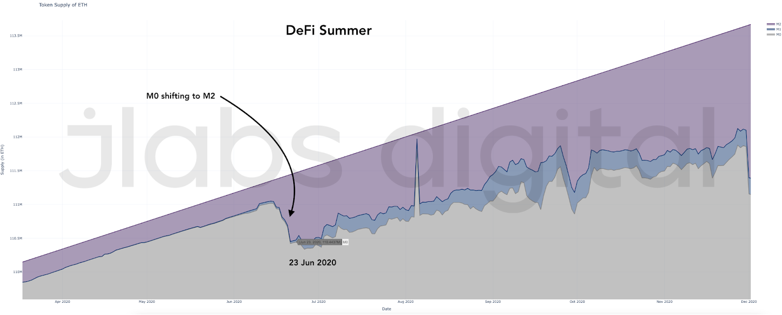
What we see is the most liquid form of ETH, as measured by M0, fell fast. ETH went from its lower form of usage to a higher form as shown by the expansion of the number of ETH being reported as M2.

For Compound, the launch of COMP incentivized users to lock up their ETH as collateral. It was a major shift in use case for ETH that rippled out to other protocols.

In turn, this changed ETH’s responsiveness to changes in supply and demand. In the most basic sense, the decision to lock up ETH into a contract to then borrow against that collateral meant the decision process to sell the token changed as well.

It was no longer sitting in a wallet that could be sold… It was now being used to borrow against. This required depositing the tokens into a smart contract, having a collateral-to-loan ratio, and paying a borrowing rate.

This usage as collateral was a higher form of ETH versus it sitting in a basic wallet.

Now, price didn’t respond right away. Remember, changes in money supply change how responsive a token’s price is to a shift in demand or supply.

If we are talking about a token’s response to demand being more sensitive, then any uptick in demand can create outsized movements in price.

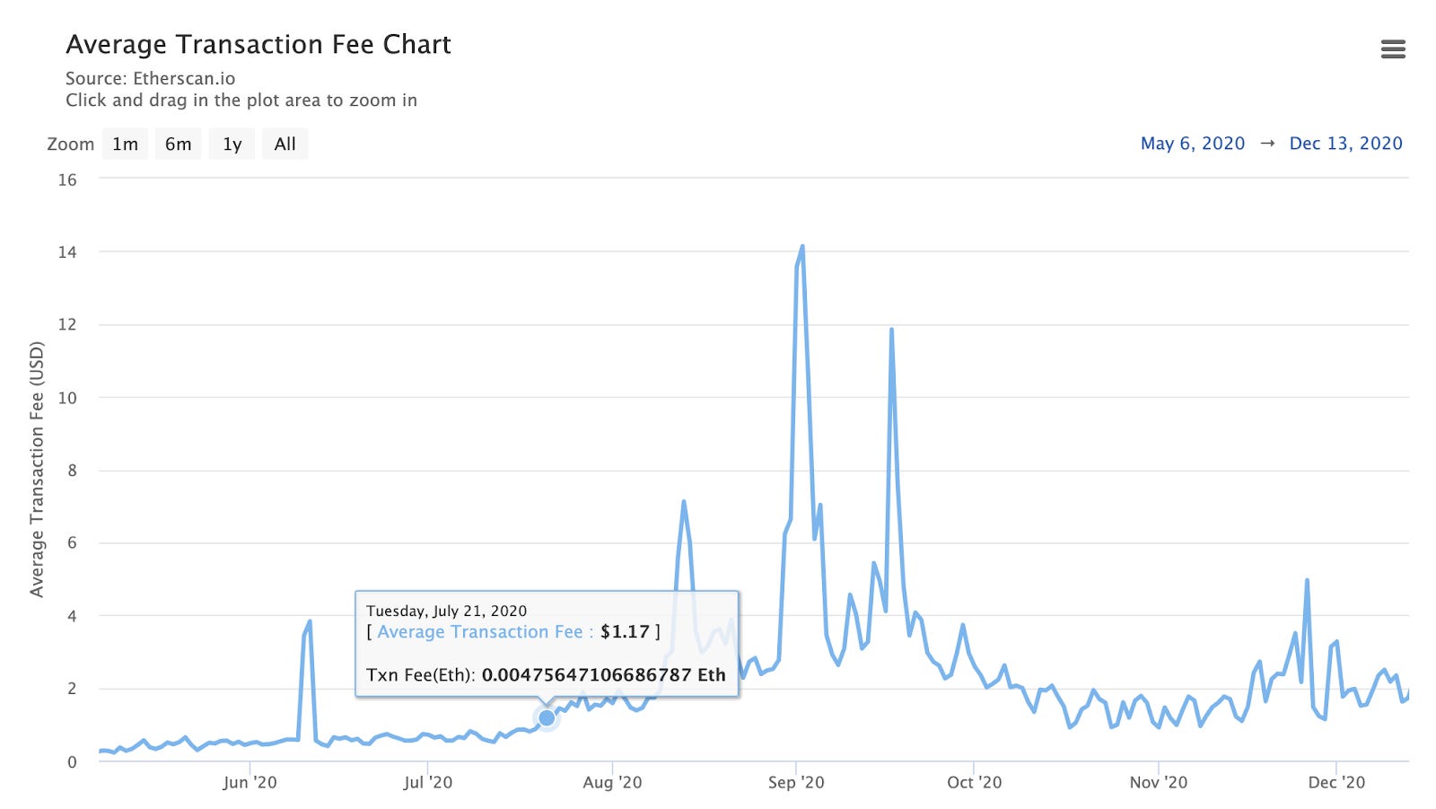
To show the importance of this, we can look at the network activity rising. Remember, conditions were set for a significant response in price with an uptick in demand.

Here’s the date of the uptick in network activity.

Here is the movement in price relative to the token becoming more sensitive to price (ETH shifting from M0 to M2) and the catalyst of demand in the second vertical line.

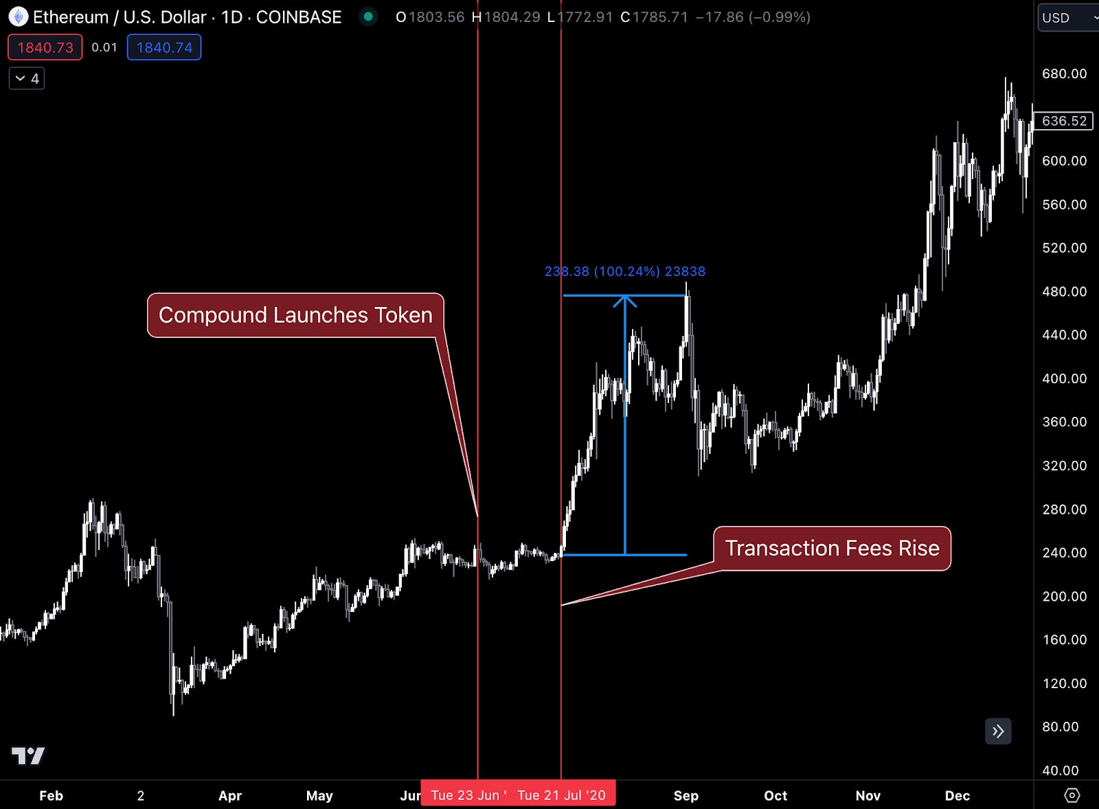
A 100% move on price is pretty substantial.

Now, I’m showing you this token supply change followed by a catalyst to show the significance of token supply in this equation. It’s like turning the car engine on before the catalyst of you hitting the gas pedal.

The catalyst part we will dive into more later as I really don’t want to go into the weeds on that just yet. I’d rather focus solely on token supply changes shifting and creating the conditions for major moves in price.

It might seem long winded, but we are going step by step here.

And if you’re feeling a bit lost, here is a mental model of where we are going, which is applying the Quantity Theory of Money to cryptocurrencies, a version that I call the “Quality Theory of Tokens” or QTT.

Here is the Quantity Theory of Money:

MV = PQ

If we rearrange it, we get:

P = MV / Q

Don’t worry so much about it, just know that we’ve been discussing “M” for the first few essays. Once we master this variable, we can get into “V” and “Q” some more. For the curious here, the transaction activity mentioned above in network fees is “Q.” And in equation form, this model looks like this:

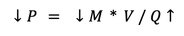
Wait, price goes down… But you said price rose 100%? Why is the arrow pointed down? Because a lower price level means an increase in purchasing power, which means less ETH needed to buy “stuff.”

Like I was saying… we will get there in time. For now, let’s stick to “M” and really unpack it before we go to the others. I just want to give us a glimpse of where we are headed with all these essays.

And to make this theory a bit easier to digest, I’ll use the same examples from today when we touch on “V” and “Q” at a later date. This will give us some continuity.

OK, back to the examples…

To sum it up here, DeFi summer happened… the usage of ETH tokens changed… And once activity appeared, the token became much more responsive to upticks in demand.

Neat. Decent explanation, but I know what you’re thinking… Are there other examples?

The Examples

To avoid this becoming overkill in terms of length here, I’ll just show the change in supply first, followed by the token’s move in price one by one. We already did our first example, so let’s get to the next.

Exhibit Two: September 2020

Here, we have a constant shifting from M0 to M2 until mid-November so that M1 (inclusive of M0) began to go sideways. This was a first for ETH. In the first example, there was a major one-time shift… Here, we have a major trend forming.

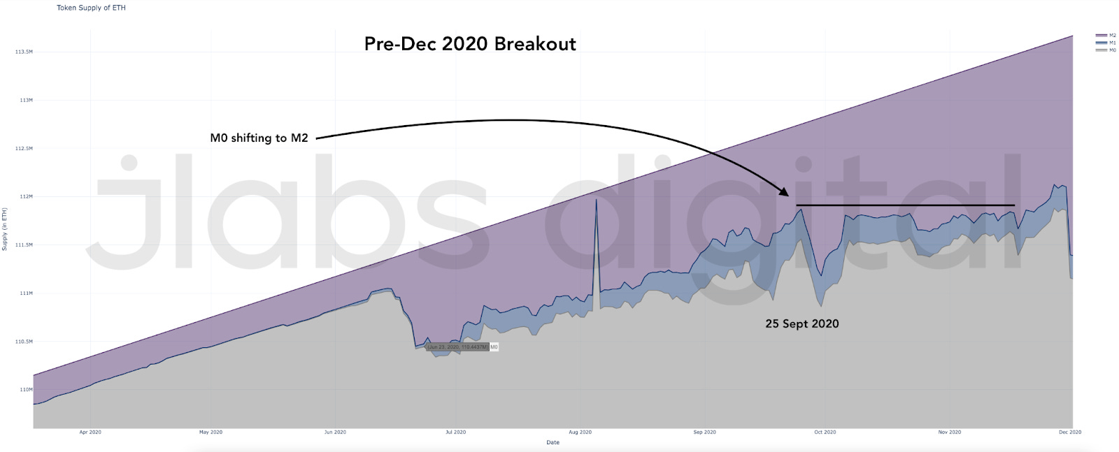
Over the next two months, price rose 75%.

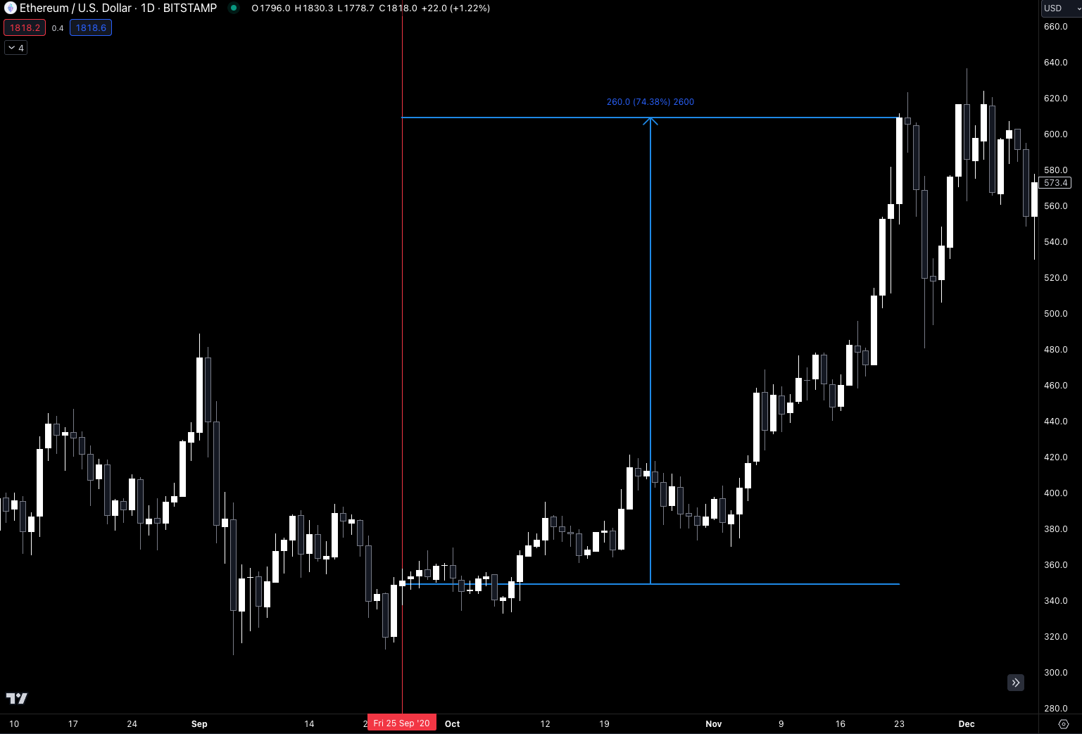
Exhibit Three: December 2020

This time around, M1 (inclusive of M0) is now declining. Another first for ETH supply. More and more ETH went toward M2 usage.

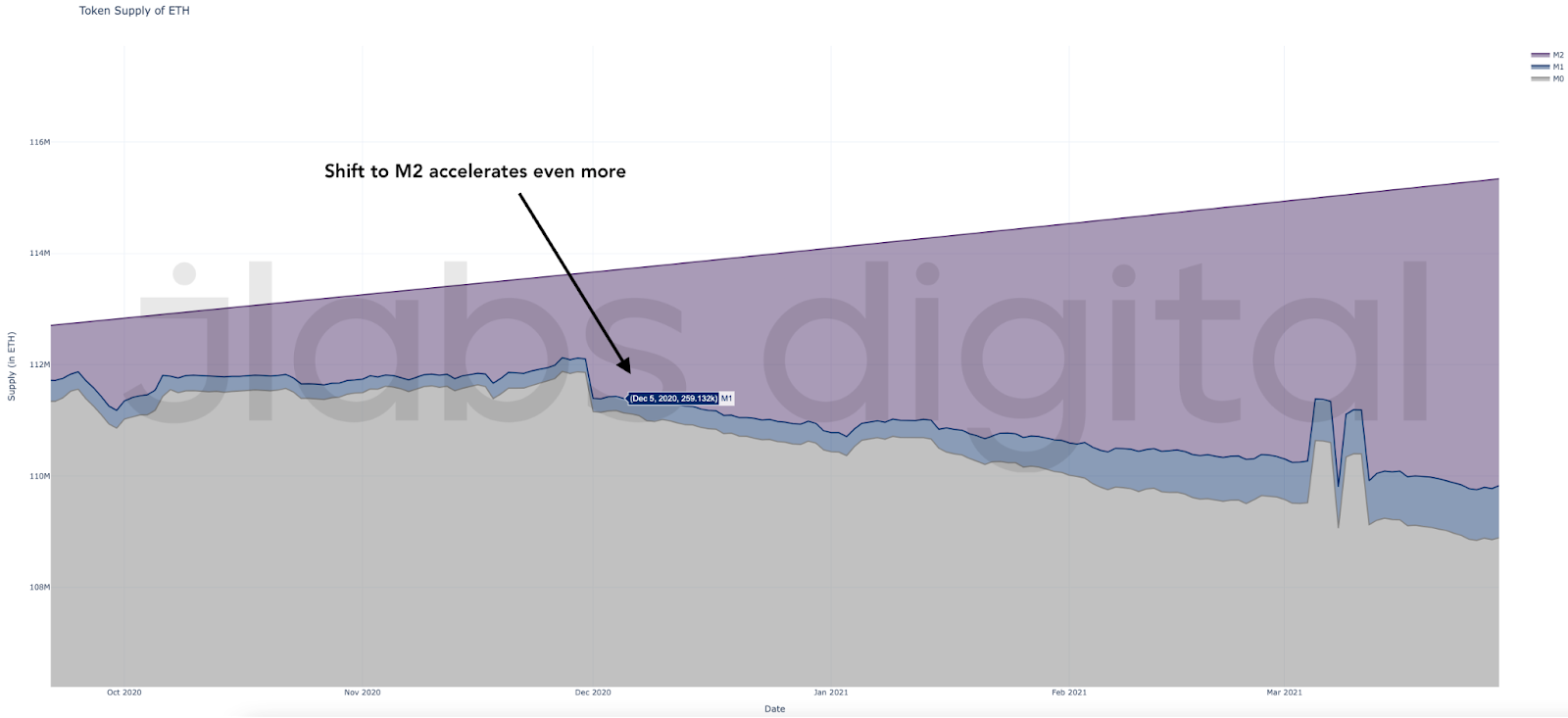
Price rose more than 100% in the next 30 days from when this decline in M1 (+M0) began (the blue brackets in the chart below). As you can see in the chart above, this trend persisted for all of Q1 2021. Price went on to rise well over 200% in Q1 2021.

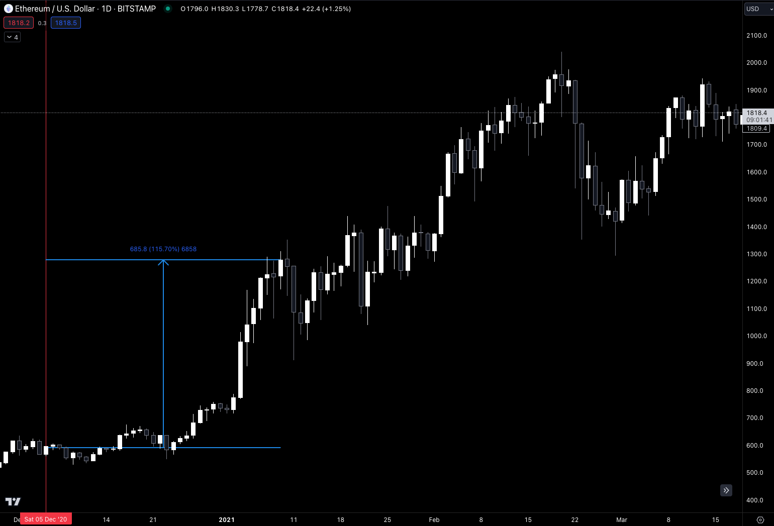
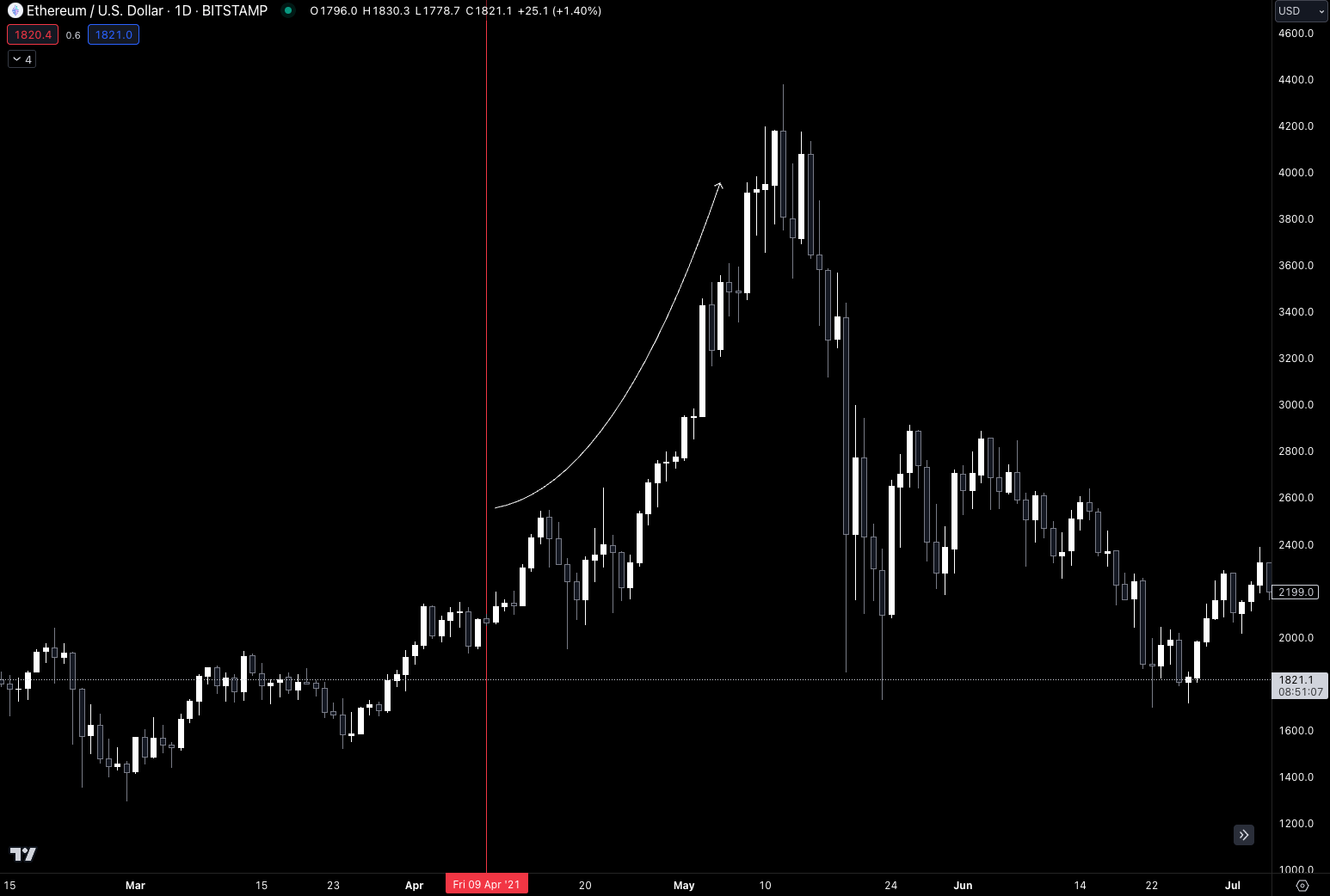
Exhibit Four: April-May 2021

On April 9, 2021, we saw the trend in M1 (+M0) make a notable drop.

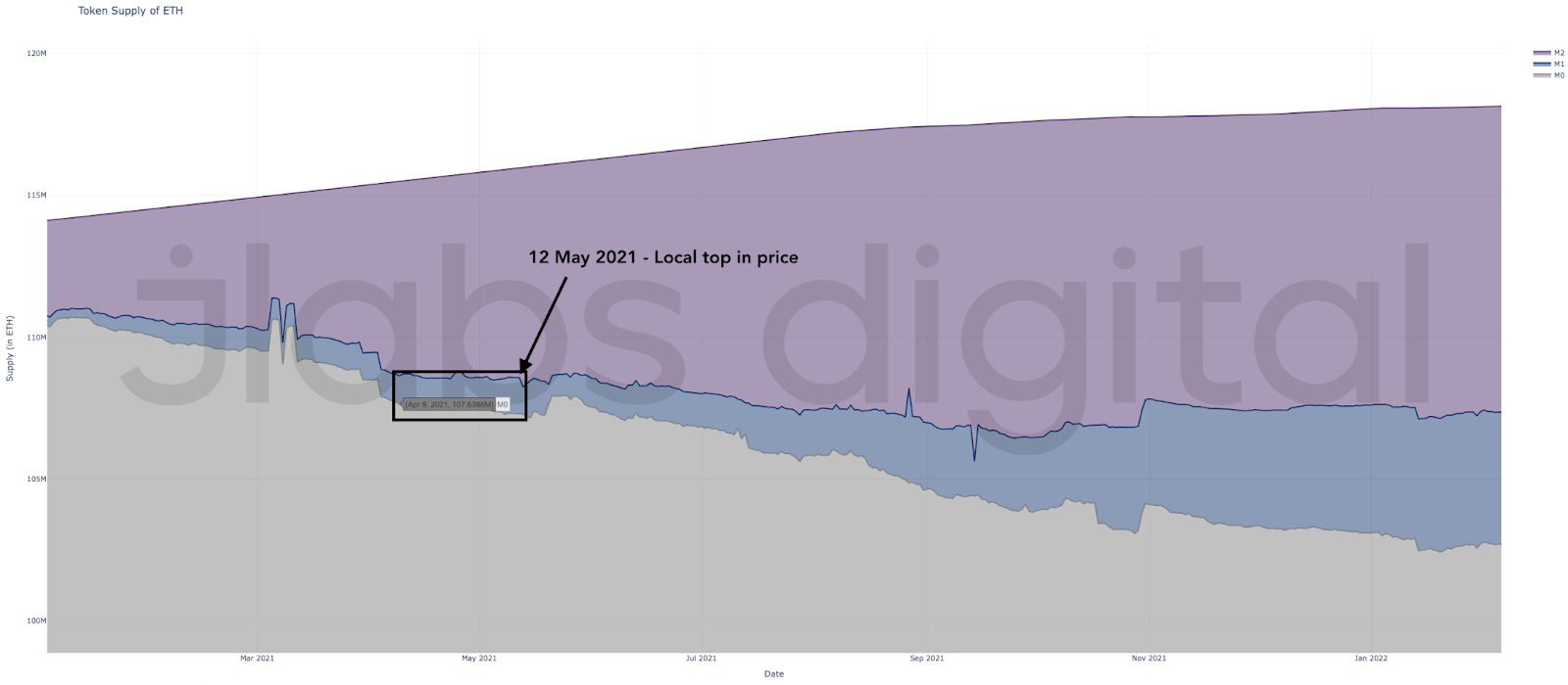
Here’s price responding in a parabolic fashion, climbing 100% over the next 30 days.

Now, it’s worth noting how price retraced rather quickly. And the supply of M1 (+M0) went sideways… There wasn’t a major increase.

This is where the equation from earlier (“V” specifically) will come in handy at a later date. For now, simply note ETH’s response in terms of price to its change in usage.

Exhibit Five: October 2021

M1 has a break in trend. This is one of the first such instances in 2021. Here we see ETH shifting to more liquid forms of usage. It’s a shift from M2 to M1.

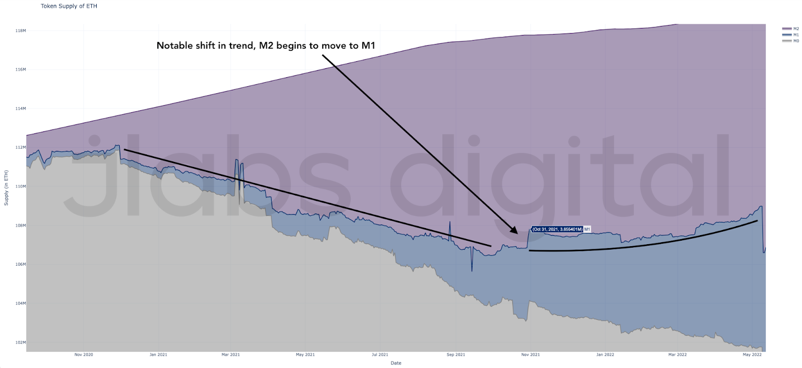
This trend change in ETH usage led to price declining in the months that followed.

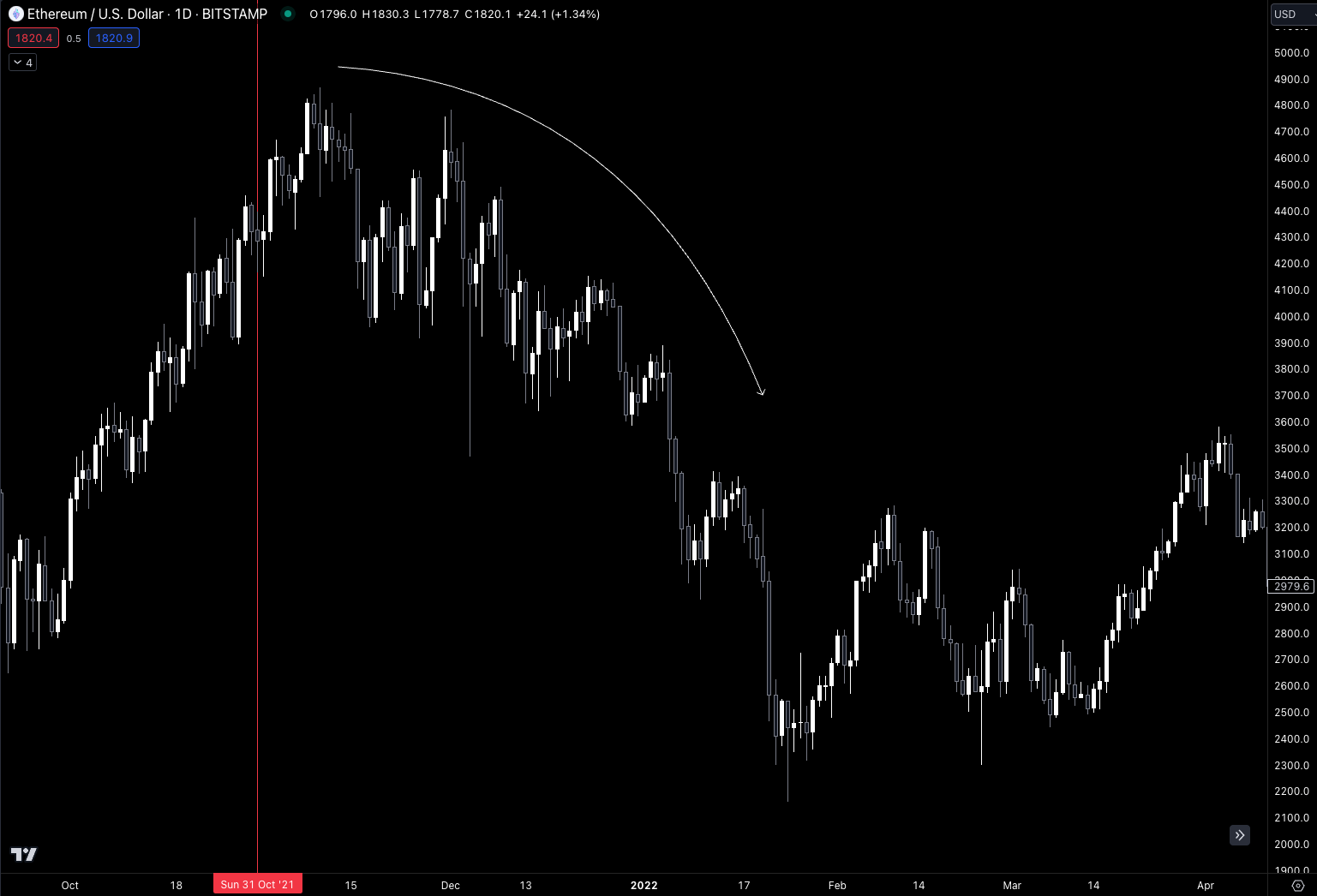
Exhibit Six: 2022

This shift in supply usage continued from October 2021 until mid-September 2022. We can see M0 went sideways while M1 continued to grow. M2 during this time fluctuated within a small range.

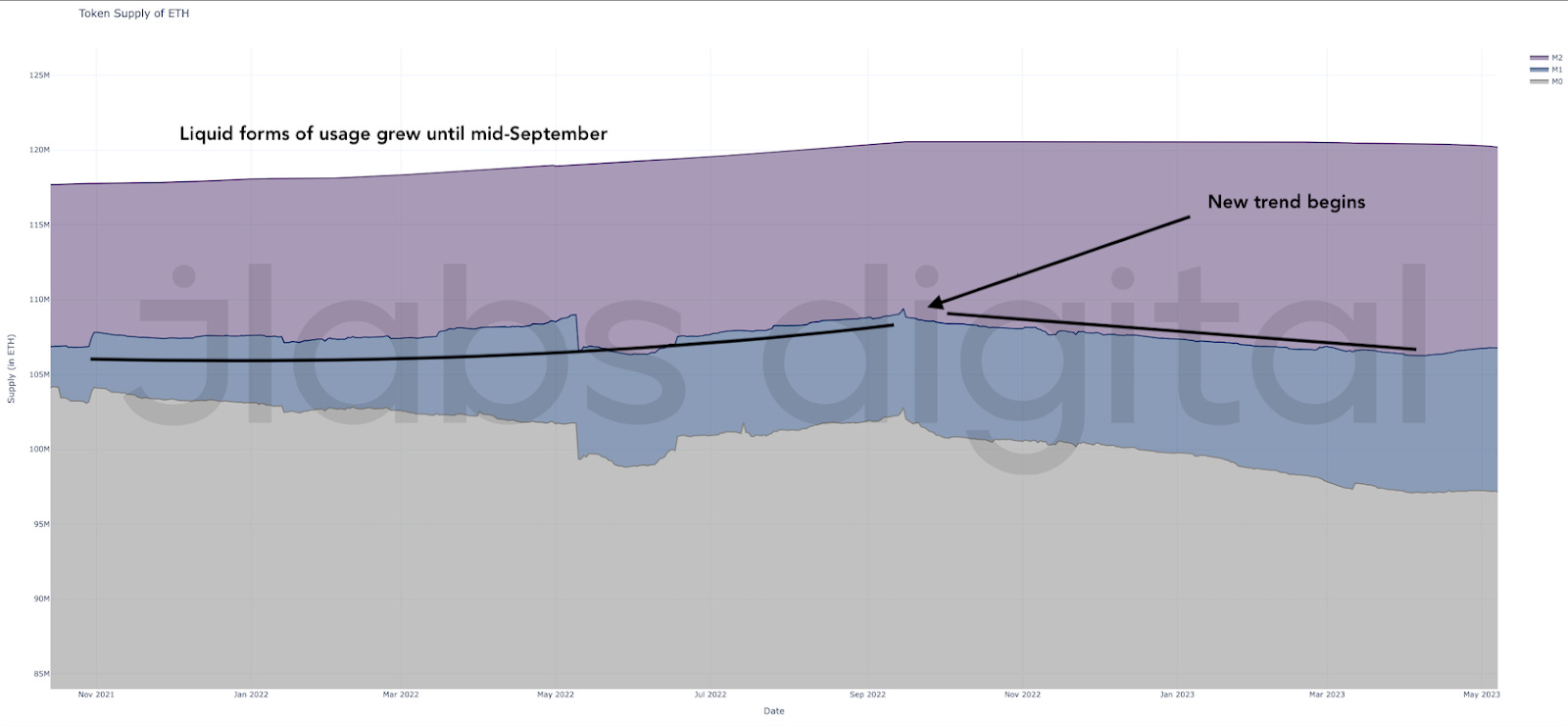
Here is how price behaved over this period.

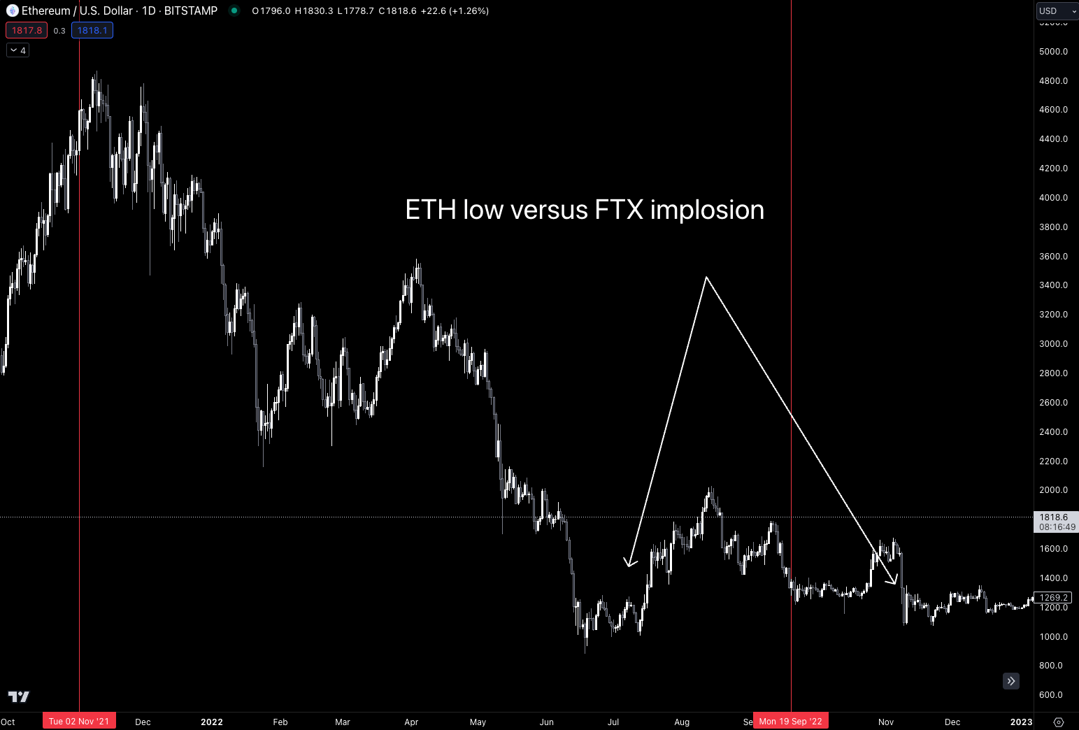
It’s important to remember FTX imploded two months after this shift came to an end. When FTX happened, ETH’s price did not form new lows for the year.

This suggests that ETH’s ability to absorb less demand as well as more sell volume was much better than before, as it shifted to a higher order of usage indicated by the growth in M2 for the month prior to the collapse.

This important dynamic, which is how ETH’s elasticity changed in the weeks leading up to FTX, becomes noticeable when we view its price reaction relative to other currencies… Even Bitcoin formed lower lows for the year during the event.

Looking at ETH’s token supply can help explain why ETH was more resilient during the selloff.

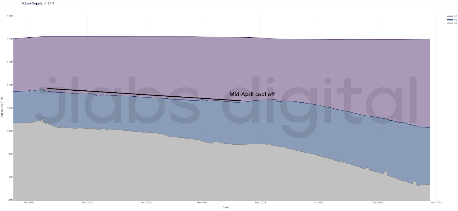
Exhibit Seven: 2023

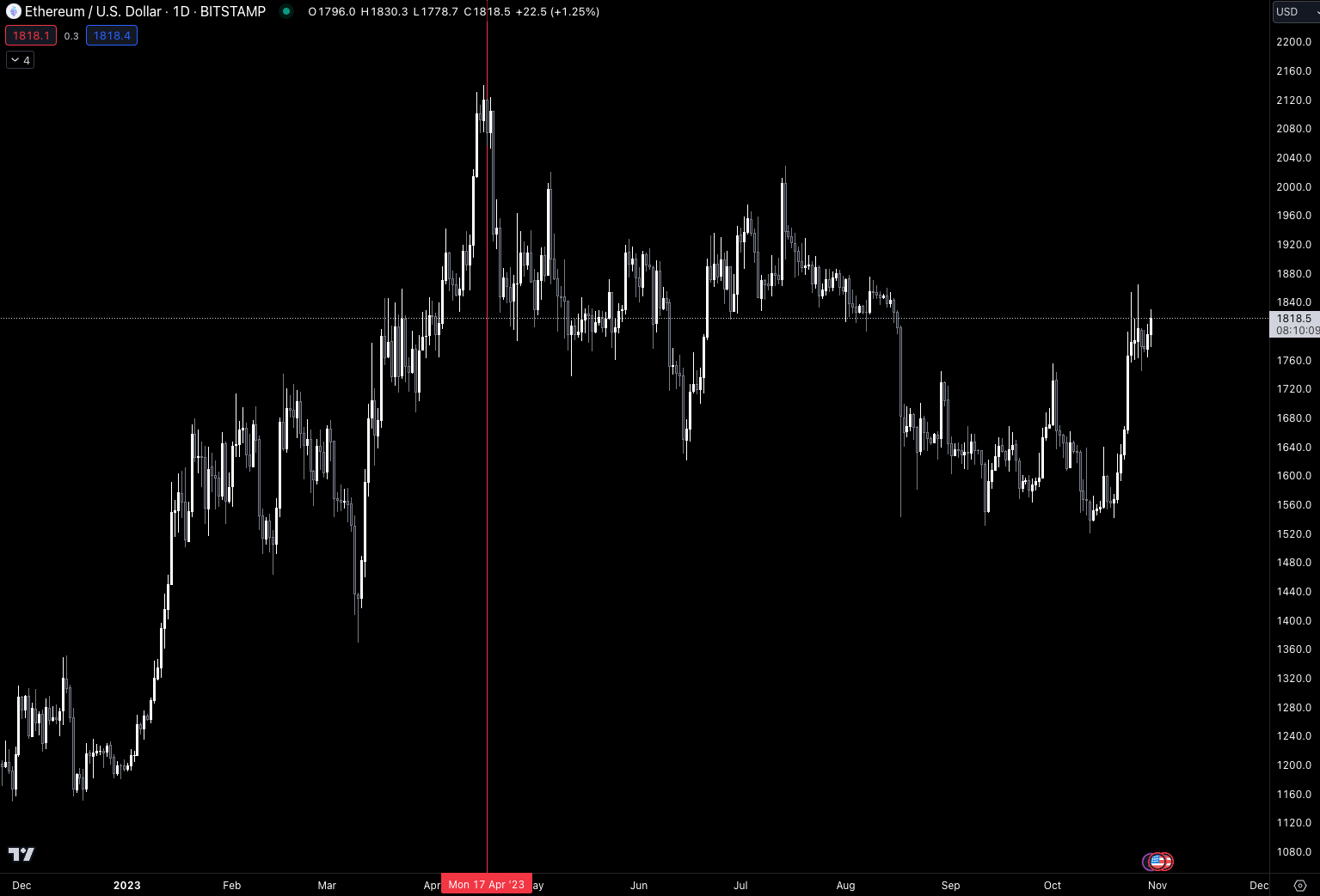
Here is 2023’s trend. We had a mild cool-off in April along with the cool-off in price action. This coincided with the Shanghai upgrade where ETH could be unlocked.

Here is the price action where ETH hit a local top.

Here is M2 by itself during that span with the same date in the price chart above highlighted.

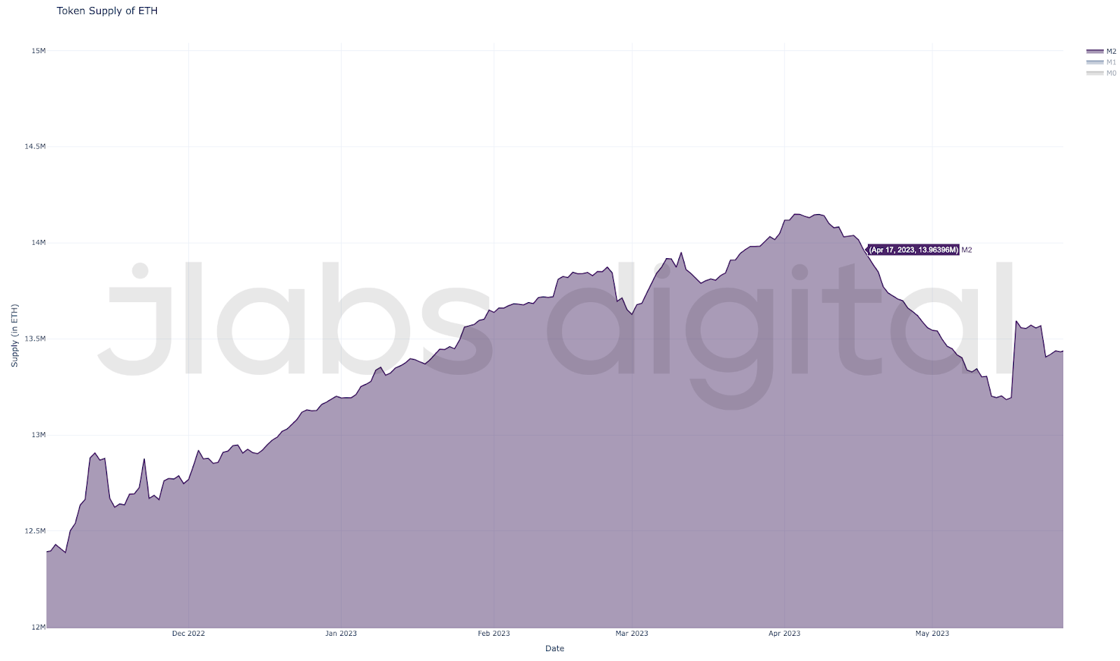
Exhibit Eight: Q4 2023

The last example here is the current trend at the time of writing. It’s going very high for M2. You likely saw it in the prior example’s chart, but I’ll go ahead and redisplay it here.

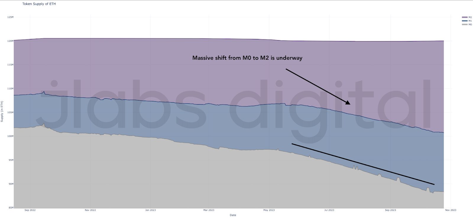
This major trend change took place during the Shanghai upgrade. The upgrade enabled unstaking for ETH staked to the Beacon Chain, which weakened the use case for liquid staking derivatives.

What is important to note is price hasn’t responded – yet. The big change in usage began on May 17. Price is currently trading at the same level as it was on that date.

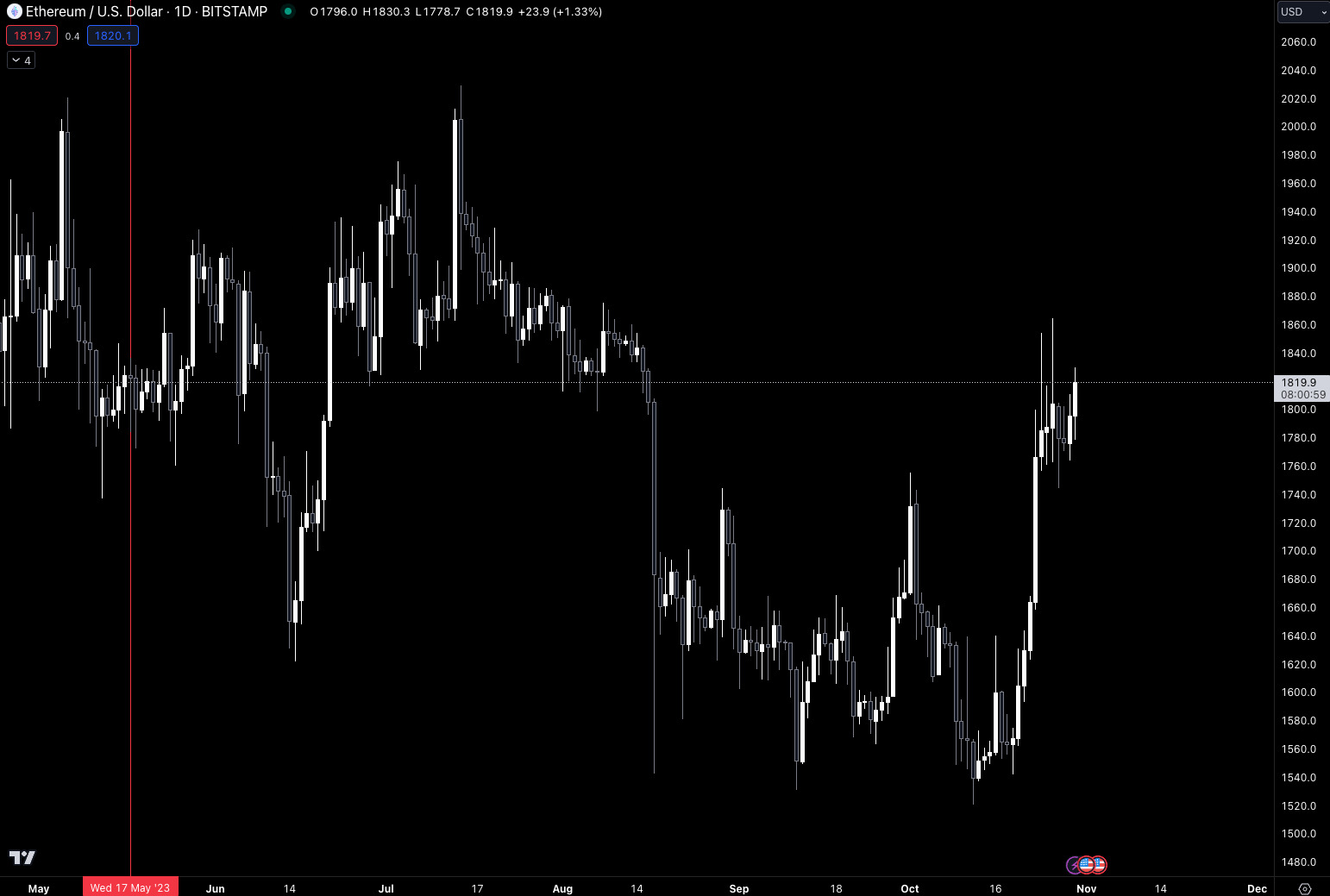
This suggests any response in network activity will likely have an outsized impact on ETH’s price relative to U.S. dollars.

We can likely come back to revisit this in the months that follow to see if this catalyst unfolded, and how price responded.

What It Means

This theory isn’t a panacea.

Many of these examples likely seem too good to be true. And I’m sure many of us here are thinking the resulting change in usage was a byproduct of some other catalyst not mentioned today.

That may very well be true.

As for this discussion here, we still have a long way to go. Specifically, we need to spend more time understanding the catalyst that sparks the token’s response in price.

To better understand this nuance, we will dive a bit into “P = MV/Q” in the next essay.

In doing so, we will get a better understanding of what drives the price of a token. And in time, this will hopefully give us an understanding of how to develop sound economics for a token.

Stay tuned to Part Four… In the meantime, keep building.

Your Pulse on Crypto,

Ben Lilly

P.S. I’d like to thank the Llamas (DeFi Llama and 0xngmi) here. Some of their data was used to plug in some gaps we had in our internal data. Our team will be finishing our own version of TVL later this year. So for those that are using the Jlabs Digital OEMS, be on the lookout for this version soon.

P.P.S. If you want to subscribe to receive future essays, please go visit espresso.jlabsdigital.com - this is our primary distribution.