A Monetary History of the United States and Crypto, 2020-2023

Note From the Editor: This is part 2 of an essay that debuted on Tuesday. We suggest you read part 1 here before reading today’s essay, if you haven’t already.

On Tuesday, we started to lay out a framework for a new “Quality Theory of Tokens.”

First, we had to explain how usage, not just supply, affected the U.S. dollar and inflation in the post-COVID era. We borrowed a few ideas from the research of economists Anna Schwartz and Milton Friedman and their seminal book, A Monetary History of the United States, 1867-1960.

Today, we’ll lean into their work some more to explain how their definitions of money supply fit into the picture – and how we can use them for crypto as well.

Let’s dive in.

Medium of Exchange vs. Store of Value

In their book, Friedman and Schwartz focused on a set of definitions of money supply that central bankers and traditional financiers use.

These terms bucket money into categories called M0, M1, M2, and M3. These are nested definitions, e.g., M1 includes the figure of M0, and then it adds another category of money supply.

Some of you may already be familiar with these terms. But without getting into specific definitions of each one, I want to focus on why these terms are useful because of their relationship to liquidity.

On either end of the scale, we have M0 and M3. M0 can be thought of as cash, dollars, and your liquid checking account. M3, on the other hand, includes M0, M1, and M2, plus it adds time deposits of up to two years, money market funds, and other less liquid forms of money.

So these definitions act as a scale for how liquid the money is.

M0 is highly liquid while M3 is not. To expand on this point, Schwartz points out:

There is a relationship between the components of these measures of money supply and how they are primarily used as a medium of exchange or a store of value. The components of the most liquid measures of the money supply, M0 and M1, all act as a medium of exchange in the economy, while the added components of M2 are used primarily as a store of value. Thus, the general idea is that there is a positive relationship between the medium of exchange property and liquidity.

In other words, M0-M3 isn’t just a scale of liquidity. It also shows how the more liquid a money supply is, the more its primary use case is as a medium of exchange. On the other hand, the more illiquid the money supply is, the more it’s used as a store of value.

The importance of this might not be that noticeable, since these definitions are being applied to robust economies across the globe.

But at their core, they help better predict how supply changes might impact an economy’s price levels, which is how countries measure inflation.

For instance, if 25% of a supply is in M0 and 75% is in M3, then lots of the supply is being held as a store of value. This means a change in supply is likely to be absorbed by its store-of-value use case. It’s said to be elastic.

The new supply of money won’t simply get spent right away, like we saw in the summer of 2021.

In that period, more like 100% of supply was sitting in M0. Which is to say, any change in supply will result in a very inelastic response for price. Inelastic here means there is no give happening. Any supply change directly impacts price… Which then leads to inflation.

Usage matters more than most tend to believe.

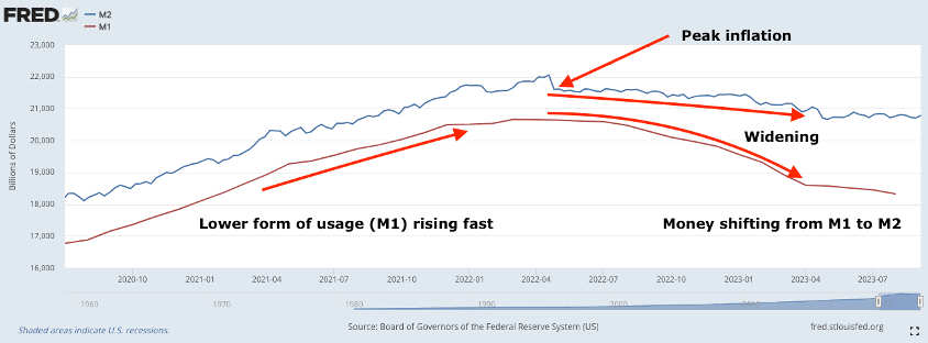
To showcase this further using money supply definitions, we can look at the chart below. We can see on the right side of the chart that in June 2022, inflation was “tamed.” What also happened here in terms of money supply definition is M1 (red line) began to shrink faster than M2 (blue line).

Said another way…

The lower form of money usage was shrinking faster than other forms of usage. The scale of usage was shifting towards M2…and money was becoming more illiquid.

Now, one quick technical note: Schwartz explains money supply based on liquidity. But I simply substitute this liquidity term for forms of usage. The more liquid money is or sitting near M0, the lower the form of usage of the money.

The more illiquid the money is or sitting near M3, the higher the form of usage. It signals an attribute related to the quality of money.

Reason I adopted this wording is mostly because liquidity in cryptocurrencies represents the amount of tokens on order books. So I don’t want to cause any unintended confusion.

OK, so here and in part one, we spent a long time going over how money is used and why that matters. Especially when it comes to the price of the currency in question. Hopefully, I’ve done a decent job at laying out these theories using legacy markets and events.

Because what I’m about to do next is introduce this same money supply definition to cryptocurrencies. Brace yourself…

Just Borrowing Things

The idea behind how to define money supply is about providing a common nomenclature. One that assists in better understanding how the usage of a currency can impact its price relative to other currencies. And hopefully, we have some agreement that a currency’s usage influences price.

Now, before we get into how I’m suggesting we define token supply, we need to hit on something many forget.

Price. It is a very nuanced term.

It can mean a lot of things to different people. For crypto, price is generally measured relative to U.S. dollars.

This causes confusion at times when a cryptocurrency is trading sideways, yet the U.S. dollar is strengthening 20–30% relative to other government-issued currencies. That means relative to other currencies, cryptocurrency is trending up.

Evaluating price based on another currency causes this issue of relativity.

It ignores whether the currency is strengthening or weakening where its usage is greatest.

In fact, if we can evaluate the strength of that currency relative to where it’s predominantly used, price becomes something else. We usually refer to price in this context as how much a dollar will buy in its main economy or country of origin. And to measure this over time, we create price indexes to better gauge if the currency’s purchasing power is rising or falling in that country.

For government-issued currencies, this is rather common. For the U.S. dollar and its economy, it’s the Consumer Price Index (CPI).

This is how we are able to measure how inflation climbed to 9.1% in the summer of 2021 spending spree.

But for a cryptocurrency, things get rather technical when we want to apply this same logic.

Specifically, how much storage or computation power can one token purchase? How much does it cost to send a transaction or change the state of the network? How does it differ now compared to one year ago? The items purchased in this economy differ from what inflation normally measures in our lives.

It might not seem important, but this context matters. For instance…

If the Ethereum (ETH) network has very high gas costs, yet its token is up 50% relative to the dollar… it’s easy to see why such knowledge is helpful when discussing whether the price is higher or lower. After all, relative to dollars, the token is stronger. But relative to the economy where it’s used natively, it’s down.

And knowing that a token’s purchasing power is falling directly impacts how productive builders or users on the network can be.

In this scenario, we are saying ETH’s purchasing power on the network is declining if it can’t buy as much storage or computation.

For a builder trying to make a profit, their cost to deploy a smart contract or send a transaction became higher. Their margins got tighter. It’s similar to the cost of gasoline rising when trying to transport goods to a destination. It inhibits production.

And we are discussing this rather fringe idea here of analyzing the token’s usage in its native environment for a specific reason.

It helps us realize what we should focus on when it comes to a token’s monetary characteristics. Focusing on the token relative to itself not only abstracts away price relativeness, but lets us better measure whether the token’s purchasing power is higher or lower.

Measuring the spending power of a token is how we measure a network’s inflation rate. (It’s basically CPI but for a network. We will showcase this metric again and dive into our methodology some more in a separate essay).

But what this mental framework helps us do most is realize how important it is to look at a token in its native format.

We see this done with the U.S. dollar. It’s measured relative to itself… And yet, we still try to compare each token to the dollar. This causes unnecessary confusion.

If we analyze a token through its native units, we can then step back and better gauge how it will behave relative to other currencies.

It is our opinion this is best done using the existing definitions of M0-M3, but tweaking them for tokens.

To be specific, we apply M0-M3 in the following manner that reflects lower to higher forms of usage:

• M0 is supply sitting in a wallet.

• M1 is supply sitting in a smart contract and acts as market liquidity. These are smart contracts like swap contracts for a decentralized exchange. These also include tokens that are staked, but liquid (e.g., liquid staking derivatives like stETH).

• M2 is supply sitting in a smart contract that is not as liquid, requiring an action to unlock. This can be tokens that are being lent out, used as collateral, or staked natively to the chain without a liquid form of the token.

• M3 is supply sitting in a smart contract that requires time and an action to become liquid. Examples of this are tokens locked in escrow or tokens being vested.

These definitions help us bucket tokens into various forms of usage (or liquidity, as Schwartz describes). M0 is the lowest form of usage. And within that bucket, we can further define supply by adding time-weighted analysis to the last time tokens were sent or received (hodl statistics).

Then, further up the usage tiers, we have higher forms that can produce yields like what we see with U.S. Treasuries.

Defining token supply in such a way, we are able to see the predominant usage of a token by the network.

Oftentimes, we tend to view the amount of tokens locked on a network without consideration of the units they’re being measured in or how liquid the tokens are in the market.

Tokens locked up in a swap contract are arguably more liquid than tokens that are staked to a protocol. This is why denoting both instances of the tokens as locked ignores how the token might influence price. The same logic applies when a staked token becomes a liquid staking derivative…

We are unable to see how the usage of a token might impact price if we don’t separate their usage into various buckets. And that’s why we employ these definitions at Jlabs Digital, and hope the wider market sees their merit and does the same.

This Is Just the Beginning

In part 1 of this piece, we showed you how money usage is what truly drove the wild swings in inflation, not so much the growth in the money supply.

And today, we honed in on exactly what that means, using a set of definitions that frame supply in terms of liquidity or usage.

The real advantage is in figuring out how to apply these principles to crypto.

This mindset is helpful in better understanding how elastic/inelastic a token’s supply is because we can gauge its usage. Which means we can better understand how a token’s supply might change through changes in its utility, upcoming token unlocks, or even government proposals.

This mutual understanding of a token’s usage is how we can better assess how valuable a token is or isn’t, and even better understand how a project founder can inject greater price stability into its designs.

This might seem rather grand in claim, but in essays to come, we will expand on these definitions more. I already alluded to how we can better view CPI or network inflation rates from viewing tokens relative to themselves.

We can also better assess credit markets for a token… look at how valuable a network is… anticipate devaluation events… better understand token unlocks and their impact on price... generate greater network productivity… and so much more.

It simply starts with abstracting away relativity. Once that’s done, we can better assess the quality of the money or token in question.

More to come. Until next time…

Your Pulse on Quality Crypto,

Ben Lilly